It’s All About Efficiency

Faster than any other area of human endeavour in history – computer technology is constantly evolving. It’s not an exaggeration to say that every month, the developments in a certain field yield at least one more option to experience the digital sphere, one more newer and better way to look at the world itself.

As a computer science expert, you might be sceptical about trends and brands. We are too – and we get it. More often than not, the product stays the same. Only the package has been modified. However, there’s one thing you shouldn’t be sceptical about: efficiency. As far as we are concerned, efficiency is what makes the difference. And the only thing you should look for every time a new tool evidently disrupts the market. Let us illustrate the point.

You can develop the front-end of your website in Notepad, can’t you? Would it be fast? Would it be convenient? Can we make this any more clear?

You can apply the same test – let’s call it the Notepad-test – to determine whether you need a new tool no matter what the field is. Machine Learning (ML) certainly isn’t an exception. Say you’re already comfortable with a certain IDE. Why would you want to switch to a new one? There’s no other answer to this question other than efficiency. The only reason to go out of your comfort zone is due to more comfort. And, regardless of the IDE you’re used to, Azure ML Studio might just offer you exactly that.

What’s So Special About Azure ML Studio?

Let’s start with three simple questions.

First question: which are the two basic components of ML?

Loosely speaking, the answer is data and computer power. There’s no need of ML without the former, you can’t process it without the latter.

Second question: why do humans hate large sets of data so passionately?

Data is usually all about numbers and figures and human brains are usually unable to process either easily.

Third question: how do we bypass the problem?

One word: visualization.

If you know anything about Microsoft Azure, it’s probably that it’s one of the two most popular cloud computing services out there. You may have wondered whether it’s your best bet, or even if you should migrate your business to Azure. But not much more.

However, things have changed, and the popularity of data science and ML has contributed to it. And if there’s one more reason to get an Azure subscription – Azure Machine Learning Studio is certainly that reason.

Here are six things you can do with Azure ML:

use a virtual machine of your choice on pay-as-you-go terms and conditions;

create and manipulate numerous SQL databases

leverage data visualization

codelessly – if you don’t want to deal with ML algorithms;

if, nevertheless, you want to – create your own ML algorithms and sell them: just visit the Azure marketplace;

while you’re there, you might want to browse carefully: there are numerous sample projects and datasets of which you can take advantage.

Still not convinced?

Let’s be a bit more practical and look at Azure ML Studio in action.

Using Azure ML Studio to Learn More About ML

The first step is, obviously, creating the Azure subscription. Don’t worry: it’s free. You may want to get more powerful virtual machines than the ones you get with the basic subscription later on. If so, you will have to pay about that. But only as much as you will actually use the machines (pay-as-you-go terms).

For now, no need to bother yourself with it. Or anything else other than the subscription.

So, go to Azure, sign up with your Outlook account (yes, you are going to need one if you want to work with Microsoft’s services; and Azure is one of them), and create a new subscription for free.

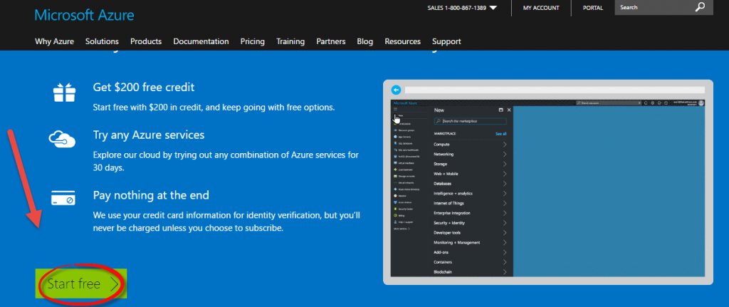
After the subscription has been created, visit Azure ML Studio and sign in with your Azure account. As easy as that.

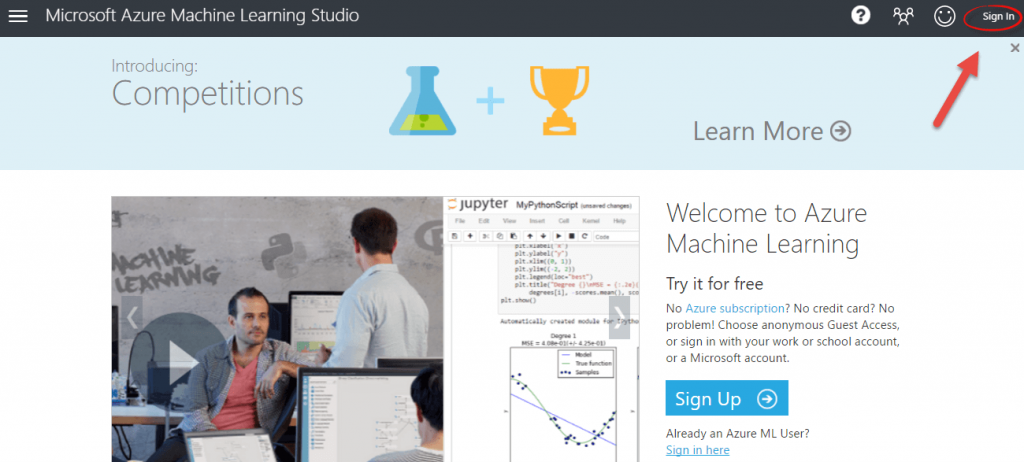
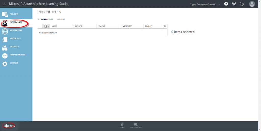
Welcome: this is your future workplace. On the left-hand side, you will instantly see few buttons: Projects, Experiments, Web Services, Notebooks, Datasets, Trained Models, and Settings. We’re interested in creating a new Project.

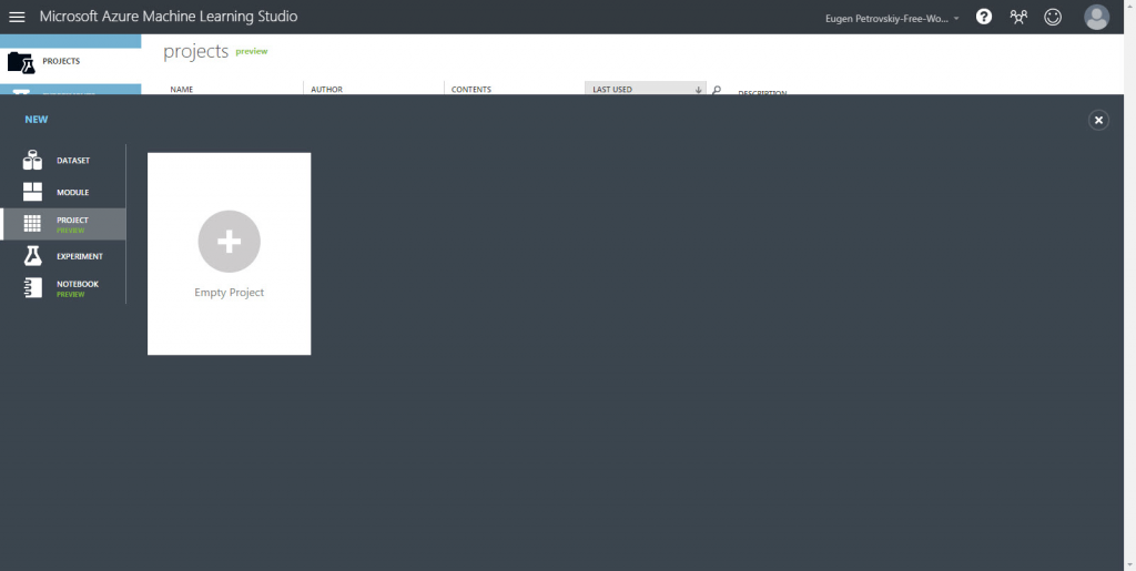
Name it anyway you want to and put in a few words as a description.

Now, we’ll need to experiment a bit. The “Experiments” area is where you’ll usually manipulate with data sets. So press “+ NEW” on the bottom left-hand side.

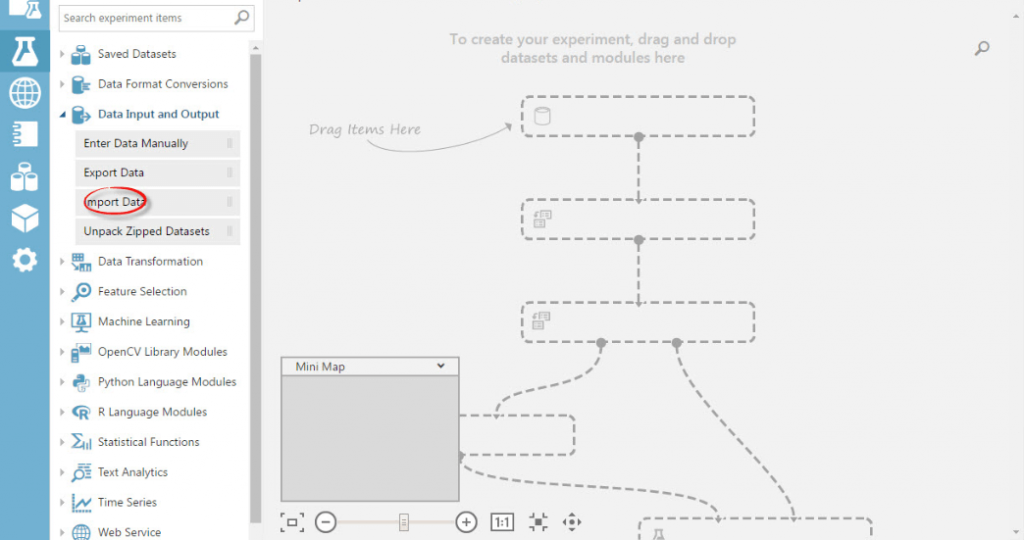
You will see an empty tree-like diagram which contains only placeholders for your future operations. This diagram can tell you a lot about how ML studio works. Adding new manipulations is as simple as drag-and-drop from the left to the right. And even easier: you can easily search experiments using a text string.

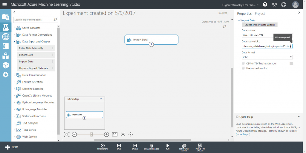
However, adding data is where everything starts. So, drag “Import Data” to your experiment.

For the purposes of our article, we’ll import open source data from the UCI Machine Learning Repository at the following link:

https://archive.ics.uci.edu/ml/machine-learning-databases/autos/imports-85.data

The file contains information about different car types. If you take a look at the data, you’ll notice that each line begins with a number between -3 and 3. Each of the numbers represents the respective vehicle’s risk factor. In the current experiment, we will try to predict the risk factor by creating, training, and evaluating a ML model using the features we have at our disposal.

If you click on “Import data” on the left-hand side of your screen, the importing properties will appear on your right-hand side. Copy the URL of the source we provided above and paste it into the “Data source URL” field.

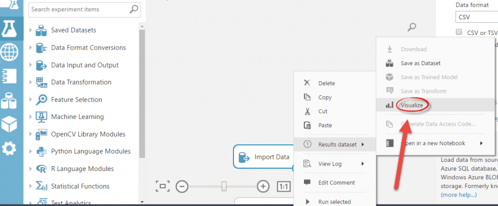
Press the right mouse button on the “Import Data” field ‡› Results dataset ‡› Visualize. This is how you will be visualizing your data sets in the future.

Once your data set is loaded, you will see not just a simple table for your data, but also relevant statistics for each of the columns.

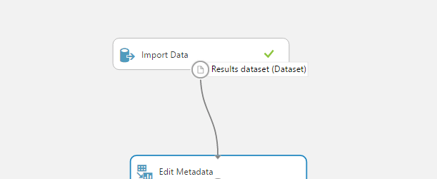
Now, let’s get back to the experiment. We need to label some of our columns to make the table more comprehensible. Go to the panel on your left side and search for “Edit Metadata”. Then, drag the field and place it below “Import Data”. To connect the fields, just press the left mouse button on the dot at the bottom of the “Import Data” field and then pull it to the “Edit Metadata” field.

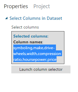
Go to the properties for the “Edit Metadata” field. To label the fields, press “Launch column selector” and pick the following columns: Col1,Col3,Col8,Col12,Col21,Col22,Col26.

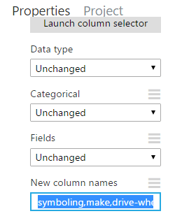
Now scroll to the field titled “New column names” and insert there the following string: symboling,make,drive-wheels,width,compression ratio,horsepower,price.

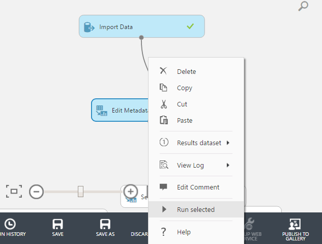
To perform labelling, press the right mouse button on the “Edit Metadata” field and then click “Run Selected”. Both the current and the previous field should become highlighted. After it’s over (green toggles should appear in the right upper corners of the fields), you’re ready to visualize your data. You will now see that the columns are labelled appropriately.

Let’s select the columns that we need. Search for “Select Columns in Dataset” and drag the module into the experiment. Then, create a connection between this module and the “Edit Metadata” field. Click on “Select Columns in Dataset”, launch the column selector, and then choose the labelled columns.

In order to prevent false results, we need to clean our data a bit. You know the drill: search for the “Clean Missing Data” item and drag it to the experiment. Connect it to the previous column and edit the properties. You’ll be selecting the columns by type “Numeric”. The minimum missing value can be 0, while the maximum missing value allowed is 1. Set “Cleaning mode” to “Remove entire row”.

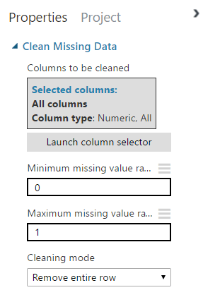
Run it and visualize the data. Now, the table should contain no empty columns.

As you may have noticed, every time you press “Run selected”, the action is applied on all the fields, not just the current one. However, there’s something you can do with this now. Click on the “Clean missing data” field. On the bottom panel, you will see a “Save as” option. Press it.

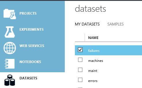
You have saved your first dataset. You will be able to access it anytime, for this or any other project. You can find it under “My Datasets”.

Drag it to your experiment. Visualize it to make sure it’s the same data you got after labelling and cleaning.

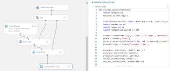
Now that we went through all the preparatory steps, it’s time we get back to our objective. In case you forgot, we needed to create a working model which will help us to predict the risk level for vehicles we may want to test later, based on information about previous cars. In order to do this, we’ll need to add just 4 more blocks: “Multiclass Decision Forest”, “Train Model”, “Score Model”, and “Evaluate Model”. Afterwards, the project should look something like this:

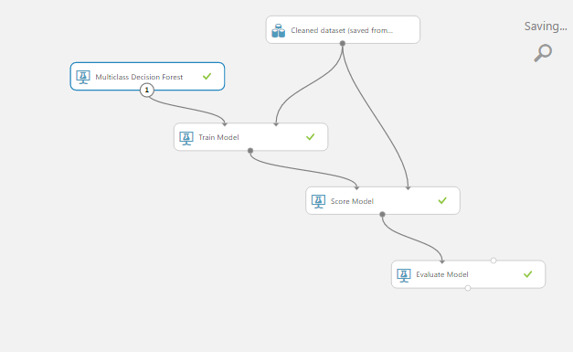
In the “Train Model” module, launch column selector, and pick “Symboling”.

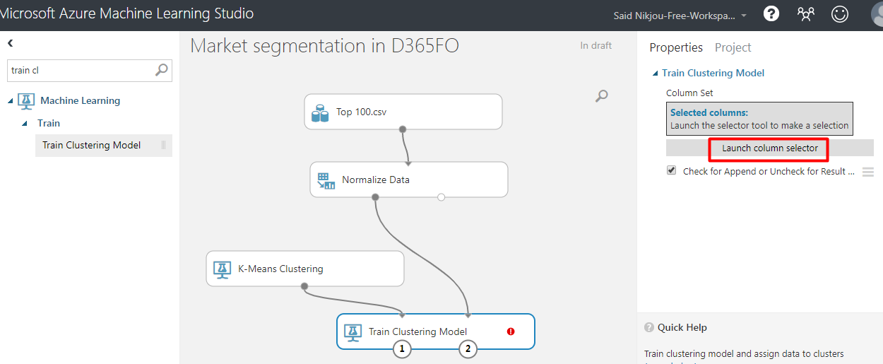
Make sure that your data set is connected to both the “Train Model” and the “Score Model” fields at the same time. Click on the “Evaluate Model” field, and then “Run selected”. Visualize your data. You should see the “Metrics” and the “Confusion Matrix” fields. Now you can see how accurate our model actually is.

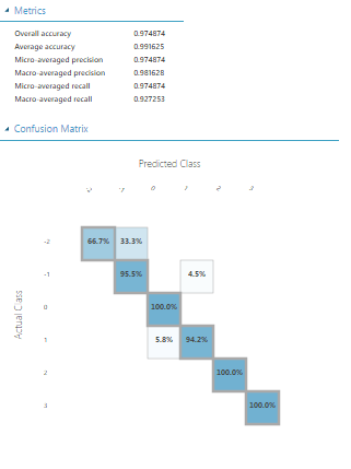
You can retrieve this data with the help of the R or Python script (first you will need to add “Execute Script” item from the left side panel).

And that’s it.

Following our instructions, you have managed to create and train a model with a high predictive accuracy without any scripting. If you found it interesting, you shouldn’t stop here: we highly recommend that you take a look at some of the sample projects on Azure’s website and learn more about the best ML practices.

Conclusion

The ability to reason over data to create intelligence is the future of computer science and humanity as a whole. Microsoft CEO Satya Nadella phrased this as clear as possible, when he described the mission behind Azure’s smart services in the following manner:

 

We are building out our infrastructure to … empower every developer to be able to infuse intelligence into everything that they are doing.

Microsoft CEO Satya Nadella

But, don’t get ahead of yourself: as useful as ML studio is, it won’t make you a proficient data scientist. First of all, you’ll need to learn more about ML and some of its basics. And then, you’ll need to better understand which algorithm you should use for which case and why.

Nevertheless, if you want to get there, Microsoft Azure ML Studio may be the way to start. Azure services are specifically designed so they can help you develop your skills and get to a more advanced level significantly faster than you may be able to do it on your own.

We tried it. And we like it. It’s your turn.